By Brian Hayes
How many passengers can the nation’s airlines carry between all the pairs of cities they connect? How many gigabits of data can pass through the optical fibers that make up the backbone of the Internet? How much electricity can the power grid transmit from generating stations to customers? From the point of view of theoretical computer science, these questions can all be seen as variations on a single problem known as all-pairs max-flow, or APMF. The computational challenge of APMF is not just to solve the problem but to find the most efficient algorithm for doing so — the method that yields the correct answer with the least investment of computational effort.
Finding the maximum flow through a network has been a core problem of computer science since the dawn of the discipline in the 1950s. For some 60 years the best algorithms for APMF required computation time proportional to n3 or more, where n is the number of nodes in the network. But now a new attack on the problem, carried out by Debmalya Panigrahi, Professor of Computer Science at Duke, along with five colleagues from other institutions, has reduced the time required to just slightly more than n2. This is a huge improvement. If n is 100, the cost of finding a solution falls from n3=1,000,000 to n2=10,000. It’s an advance no one saw coming. Prasad Raghavendra of the Simons Institute for the Theory of Computing described it as “an algorithmic surprise.”
To see what makes the max-flow problem interesting, look a little more closely at the airline example. To calculate how many people can fly from Boston to Miami, it’s not enough to count the seats on direct flights between those cities. Passengers could also arrive via stopovers in Raleigh or Atlanta, or even by a roundabout tour touching down in Detroit and St. Louis and several other cities. All of these routes contribute to the total flow. And there are further complications to keep in mind. If a route includes flights on different aircraft, the seating capacity of the smallest airplane sets a limit that applies to the entire route; for this reason a max-flow solution can leave seats unfilled on some flight segments.
When looking at max-flow from a computational perspective, we can strip away inessential details and define the algorithm on an abstract mathematical structure called a graph (Figure 1), often represented visually by a drawing of dots joined by line segments. More formally, a graph consists of n vertices (the dots) and m edges (the line segments). Each edge links a single pair of vertices. Each edge is also assigned a weight, a number representing the maximum flow that edge can carry. For max-flow problems, the graph must be connected, meaning that you can get from any vertex to any other vertex by following some sequence of edges. A connected graph must have at least n–1 edges; the upper limit on the number of edges, attained when every pair of vertices is connected by an edge, is n(n–1)/2.
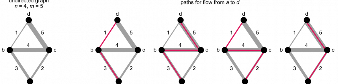
Figure 1. A mathematical graph consists of vertices, represented here as black dots, and edges, shown as gray line segments connecting pairs of vertices. The structure of a small graph is shown at left: Four vertices are joined by five edges. Each edge is assigned a weight, indicating its capacity for carrying flow. The line widths are proportional to the weights. The diagrams at right show the four possible paths from vertex a to vertex d.
The simplest version of the max-flow problem, called (s,t) max-flow, considers only the flow from a single source vertex s to a single terminal vertex t. The best algorithms for (s,t) max-flow have a running time that’s roughly proportional to n2. In the argot of computer science, they are said to have time complexity O(n2 ). (This “big O” notation ignores everything but the fastest-growing term in the expression for the running time. For example, n(n–1)/2 qualifies as O(n2 ).)
For the all-pairs version of the max-flow problem (Figure 2), the obvious strategy is to apply an (s,t) algorithm to every possible pair of vertices. There are O(n2 ) such pairs, and so it appears we must repeat an O(n2 ) algorithm O(n2 ) times, for a total time complexity of O(n4 ).

Figure 2. The all-pairs max-flow (APMF) problem asks for the maximum possible flow between every pair of vertices in a graph. The 4-vertex graph has 6 such pairs, with max-flows that range from 5 to 7. A new algorithm devised by Debmalya Panigrahi and colleagues reduced the time needed to solve this problem from Õ(n3 ) to Õ(n2 ).
In 1961 Ralph E. Gomory and Te Chiang Hu, both then at IBM Research, devised an ingenious shortcut. They found a way to take a graph with as many as O(n2 ) edges and pare it down into a much smaller graph, with the same set of vertices but just n–1 edges. This “sparsified” graph is equivalent to the original one for purposes of max-flow calculations. The edge weights of the sparsified graph are arranged so that the max flow between any pair of nodes is the same as it is in the original graph.
A connected graph with n nodes and n–1 edges necessarily takes the form of a tree. It can have branch points, where two paths diverge, but there aren’t enough edges to allow cycles, which form when two branches reunite. The absence of cycles means there is exactly one path from any vertex to any other vertex. In a tree, therefore, solving an (s,t) max-flow problem is easy: Just follow the unique sequence of edges that leads from s to t, and note the smallest weight you encounter along the way. That weight is the maximum flow for the pathway. Because this Gomory-Hu tree (Figure 3) includes such a path for every pair of vertices, it represents a complete solution to the APMF problem.

The original 1961 algorithm for constructing a Gomory-Hu tree has a time complexity of at least O(n3 ), which therefore also became the best time limit for solving the APMF problem. In the decades since then, faster methods have been found for APMF calculations on various special classes of graphs, such as those where all the edges have the same weight, or on planar graphs, which can be drawn on a plane without having any edges cross. APMF speedups are also possible if you are willing to accept an approximate solution, with a small margin of error. In the case of unrestricted graphs and a demand for exact answers, however, there was no substantial progress on lowering the exponent below O(n3) until Panigrahi and his colleagues announced their result late last year, bringing the time complexity down close to O(n2 ).
How does the new algorithm achieve this speedup? A key innovation is to abandon the (s,t) max-flow procedure as the basic building block of the all-pairs computation. Instead of calculating the flow between a single source and a single terminal, the strategy is to select a single source and find the maximum flow from there to all of the n–1 other vertices. But this plan offers an advantage only if all the flows fanning out from s to all the ts can be calculated substantially faster than making n–1 calls to an (s,t) max-flow procedure. Panigrahi et al. achieved that goal by introducing a new intermediate data structure called a guide tree, which is rather different from the Gomory-Hu tree. A guide tree need not touch all the vertices of the original graph, and it may include auxiliary vertices that are not part of the original vertex set. A procedure that prunes the guide trees, nipping off whole subtrees, rapidly yields enough (s,t) max-flow pairs to reconstruct a Gomory-Hu tree.
The time complexity of the algorithm is designated Õ(n2 ), with a tilde over the O. This extension of big-O notation ignores not only constant factors but also factors that include the logarithm of n. Thus a running time of O(n2 log n) becomes, in the Õ accounting, Õ(n2 ). The rationale for suppressing both constant and logarithmic factors is that they all become unimportant when n is very large. It should also be noted that the algorithm is probabilistic — it relies on random choices at certain points — rather than deterministic. Although it is certain to find the correct answer, the running time is guaranteed only “with high probability.”
The new algorithm is described in a paper posted on the arXiv preprint server in November 2021; it was presented in November 2022 at the annual Symposium on Foundations of Computer Science (FOCS), one of the premier gatherings of the theory community. The paper, with six authors, springs from an alliance of two groups who had earlier been working independently on various aspects of the APMF problem. Panigrahi had previously collaborated with Jason Li of the Simons Institute for the Theory of Computing and with Thatchaphol Saranurak of the University of Michigan. The second group consists of Amir Abboud and Robert Krauthgamer of the Weizmann Institute of Science and Ohad Trabelsi of the Toyota Technological Institute at Chicago.
Panigrahi thinks practical applications of the new algorithm are unlikely in the near future. Its significance, he says, is in helping to understand the complexity landscape of graph algorithms — which problems are harder than others, and why. Particularly intriguing is the connection between APMF and a closely related problem known as all-pairs shortest path (APSP). For a weighted undirected graph the shortest path between a source s and a terminal t is a sequence of edges connecting those vertices that has the smallest sum of edge weights. “It is generally believed that max-flow is a harder problem than shortest path,” Panigrahi says. “Indeed, for a single pair (s,t) the shortest path problem has been solvable in linear time for many decades while the corresponding result for max-flow is less than a year old. The new APMF result shows that in the all-pairs case, either the APSP conjecture is false or our intuition that APMF is a harder problem than APSP is false.” Resolving this conundrum and refining the APMF algorithm could be objectives of future work.
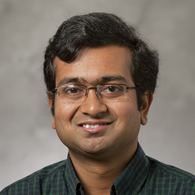
Panigrahi has been at Duke since 2013. He earned his Ph.D. at MIT under the supervision of David Karger. His earlier degrees are from Jadavpur University in Kolkata and the Indian Institute of Science in Bangalore.